In the second part of the series I am going to present you an implementation of the melody modification method I’ve described in the first part. Available here.
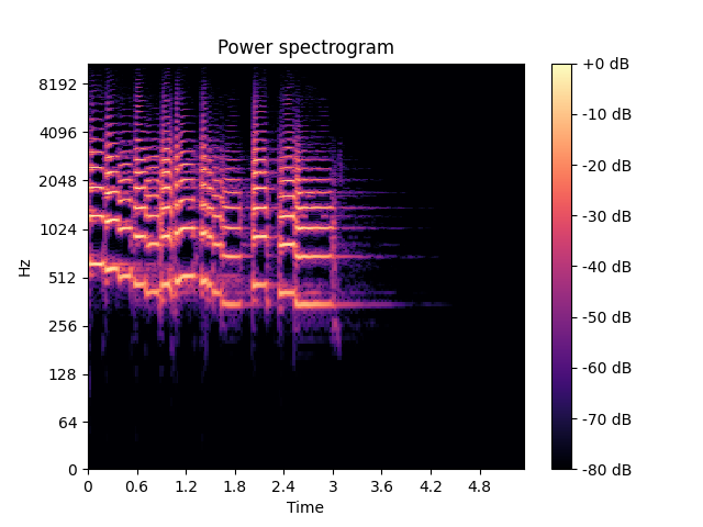
First of all, we need to have a sound sample to work on. Thankfully, librosa provides us with cool sound samples. Let’s have a look at the STFT diagram example from part I.
Code:
import librosa
from librosa import display
import matplotlib.pyplot as plt
import numpy as np

fig, ax = plt.subplots()

y, sr = librosa.load(librosa.ex('trumpet'))
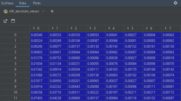
stft_absolute_values = np.abs(librosa.stft(y))
img = display.specshow(librosa.amplitude_to_db(stft_absolute_values, ref=np.max), y_axis='log', x_axis='time', ax=ax)

ax.set_title('Power spectrogram')

fig.colorbar(img, ax=ax, format="%+2.0f dB")
plt.show()

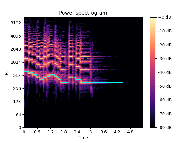
We can clearly see how the melody changes through time but the computer doesn’t know which frequency bins hold our F0 frequency information. We’re going to use pYIN algorithm implementation provided by librosa. Now let’s add F0 calculation result to the chart.

import librosa
from librosa import display
import matplotlib.pyplot as plt
import librosa.display
import numpy as np

n_fft = 4096
hop_length = 512

fig, ax = plt.subplots()

samples, sr = librosa.load(librosa.ex('trumpet'))
stft_absolute_values = np.abs(librosa.stft(samples))
img = display.specshow(librosa.amplitude_to_db(stft_absolute_values, ref=np.max), y_axis='log', x_axis='time', ax=ax)

ax.set_title('Power spectrogram')

fig.colorbar(img, ax=ax, format="%+2.0f dB")


// add f0 plot
f0, voiced_flag_t, voiced_probs_t = librosa.pyin(samples, fmin=librosa.note_to_hz('C2'),
                                                          fmax=librosa.note_to_hz('C7'), sr=sr,
                                                          hop_length=hop_length, frame_length=n_fft,
                                                          pad_mode='constant', center=True)
f0_times = librosa.times_like(f0)
ax.plot(f0_times, f0, label='f0', color='cyan', linewidth=2)


plt.show()
Let’s transform!
Now we can apply some changes to the trumpet melody. As I stated in this and the 1st part, we need to move all frequency bins from a certain point in time upwards so its tune goes up and the melody sounds higher at that point in time.
In fact, out spectrogram depicts a matrix of values where the horizontal axis describes time bins and the vertical one freuency bins.

All we need to do is roll a column (or multiple column at certain points in time) n – times up or down to change the tune. Then apply inversion of STFT to get the transformed sound. Here’s the code for column rolling. It’s quite straitforward so take a look at it:
def _roll_column(two_d_array, column, shift):
    two_d_array[:, column] = np.roll(two_d_array[:, column], shift)
    return two_d_array
Now let’s use it to actually modify the melody. I am applying the change to some columns of the trumpet melody matrix. See the code and how the plot has changed afterwards.
I am applying random shuffling to the time bins in range from 50 to 90 using code below:
img_modified = display.specshow(librosa.amplitude_to_db(stft_absolute_values_modified, ref=np.max), y_axis='log', x_axis='time', ax=ax)
ax.set_title('Power spectrogram')

fig.colorbar(img_modified, ax=ax, format="%+2.0f dB")

plt.show()
This is how the spectrogram looks like after the transformation:


We can see that frequencies have been randomly moved up/downwards in relation to the original data.
Looks promising but the change in the tune were just random and wouldn’t sound well. True, but now we have a tool which opens a broad spectrum of possibilities to modify melody that may sound really interesting!
In the next part we’re going to increase a pitch of the entire track, change the melod of human speech and of course play the sound (which didn’t happen in this article, yes I know, just be patient :)).
Hope you liked it.
In case of any questions and/or remarks don’t hesitate commenting or reaching me out!

